Feature Engineering in Amazon SageMaker Using Web Data: Step-by-Step Tutorial

In this blog post, you will learn:

• What Amazon SageMaker is and the value it brings to machine learning.
• Why web data is essential for successful feature engineering.
• Where to retrieve high-quality web data for feature engineering and other machine learning scenarios.
• How to perform feature engineering in Amazon SageMaker using datasets storing web data.

Let’s dive in!

What Is Amazon SageMaker?

Amazon SageMaker is a fully managed service built to help you build, train, and deploy machine learning models and AI applications at scale. It provides a unified, end-to-end environment for analytics and AI.

It allows you to access data from multiple sources, whether it is stored in Amazon S3 data lakes, Redshift data warehouses, or third-party and federated systems. All that while guaranteeing enterprise-grade security and governance.

In short, SageMaker simplifies ML workflows and accelerates model development, from feature engineering to model deployment. These are the main features and capabilities it equips you with:

• SageMaker Unified Studio: A single development environment for building, training, and deploying ML and generative AI models using fully managed infrastructure and integrated tools.
• Model development and MLOps: Includes prebuilt templates, HyperPod, and JumpStart for rapid prototyping, training, and operationalizing models.
• Generative AI support: Build and scale applications with Amazon Bedrock and leverage built-in AI assistants like Amazon Q Developer.
• Data processing and SQL analytics: Prepare, analyze, and integrate data using open-source frameworks on Amazon Athena, EMR, Glue, and Redshift.
• Lakehouse architecture: Unifies access to siloed data across storage systems to support comprehensive analytics and AI.

An Introduction to Feature Engineering with Web Data

Feature engineering is the process of transforming raw data into meaningful variables, called “features,” that machine learning models can use more effectively. Instead of feeding a model with unprocessed data, the idea is to create derived metrics that better capture patterns in the source dataset.

Examples include aggregating values, normalizing scores, combining related variables, or creating ratios that highlight relationships between different fields. Good feature engineering may even have a larger impact on model performance than the choice of algorithm itself. That is because well-designed features help models identify signals that would otherwise remain hidden.

Web data is particularly valuable for feature engineering because it reflects real-world activity at scale. Public websites contain large amounts of information about companies, products, jobs, reviews, pricing, and user behavior. These signals can be transformed into features such as popularity indicators, market demand metrics, sentiment scores, or hiring trends. Such features can significantly improve the performance of your machine learning pipelines.

However, working with web data also presents several challenges. The data may be noisy, incomplete, or inconsistent. This can greatly affect the quality of the input data. Plus, many websites adopt anti-bot measures.

Thus, using web scraping to power machine learning is tricky. It requires the collected data to be cleaned, validated, and prepared before it can be used in an ML pipeline.

Where to Retrieve High-Quality Web Data in Large Volumes

As you may have understood, web data plays a pivotal role in feature engineering. At the same time, retrieving it reliably and for enterprise-ready use is difficult. Collecting data from a few pages may seem straightforward if you follow a web scraping roadmap, but doing it consistently across many domains or a large site is far more complex.

Websites frequently change their structure, enforce rate limits, and deploy anti-bot protections that block automated requests. In addition, even when you manage to collect the data, ensuring that it is high-quality, complete, and up to date can be challenging.

For this reason, many organizations rely on web dataset companies and web data providers such as Bright Data. These platforms give you access to large amounts of web data so that you do not have to build and maintain a scraping infrastructure.

Bright Data offers hundreds of datasets from more than 215 popular web domains, with over 17 billion total records. These datasets contain continuously updated web data that is structured, ready-to-use, and optimized for ML and AI applications. Explore the dataset marketplace!

If pre-collected datasets do not meet your needs, Bright Data also provides Web Scraping APIs and other data collection tools. These help you retrieve fresh data from websites on demand without handling scraping challenges yourself.

What sets Bright Data apart is its data collection infrastructure. It is built upon a global proxy network with over 150 million IPs across more than 195 countries, achieving 99.99% uptime and 99.95% success rates. This foundation makes it easier to build data-driven applications and ML pipelines powered by trusted web data.

How to Perform Feature Engineering on Web Data in Amazon SageMaker

In this step-by-step section, you will be guided through the process of performing feature engineering in Amazon SageMaker.

You will start with a Bright Data Glassdoor dataset, upload it to Amazon S3, load it into a SageMaker notebook, and apply feature engineering to create meaningful metrics. Once the features are prepared, you will use them to train a predictive machine learning model for high employee satisfaction.

Keep in mind that this is just an example, and many other use cases are possible.

Follow the instructions!

Prerequisites

To follow this guide, make sure you have:

• An AWS account (even on a free trial).
• A Bright Data account.
• An S3 bucket defined in your AWS account.
• Basic Python knowledge, especially when it comes to machine learning development and data science.

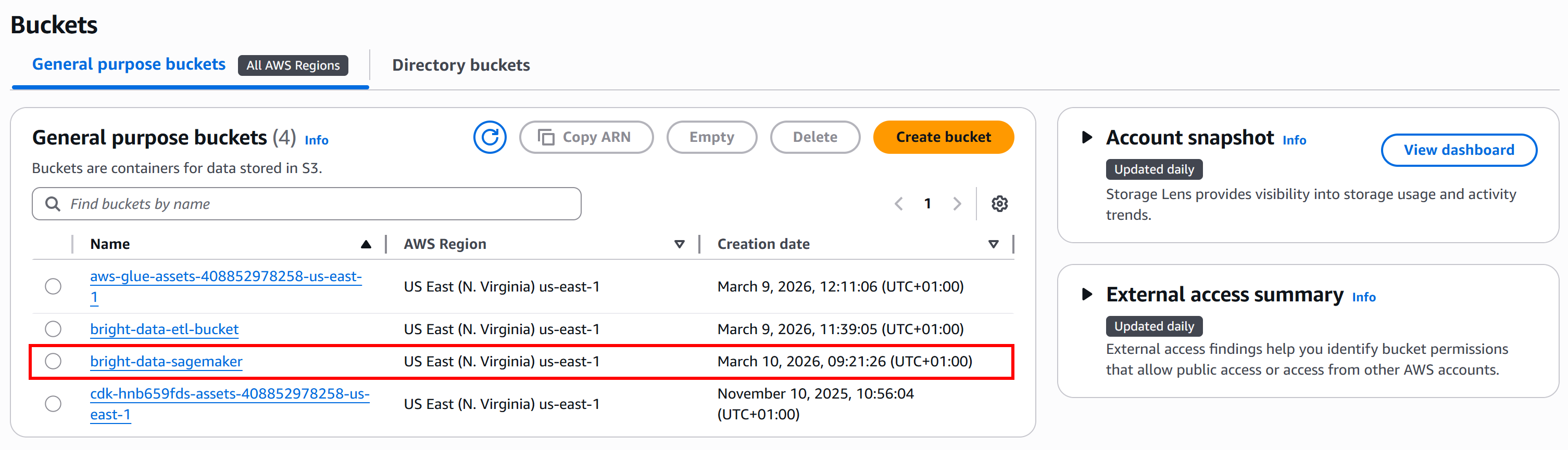
From now on, we will assume your S3 bucket is named bright-data-sagemaker:

Step #1: Retrieve the Input Dataset from Bright Data

The first step is to obtain the input web data. For feature engineering, it is best to start with a large, high-quality dataset. In this example, we will leverage Bright Data’s extensive dataset collections, focusing on a Glassdoor dataset as previously planned.

Alternative: If you prefer to collect new data, you can use one of the Bright Data Web Scraping APIs to gather fresh, structured, ML-ready datasets. These APIs offer a delivery option that can send data directly to your Amazon S3 account, making integration with SageMaker seamless.

Now, if you do not already have a Bright Data account, start by creating one. Otherwise, just log in.

In the Bright Data control panel, select the “Web Datasets” menu option. Navigate to the “Dataset marketplace” tab to browse available datasets:

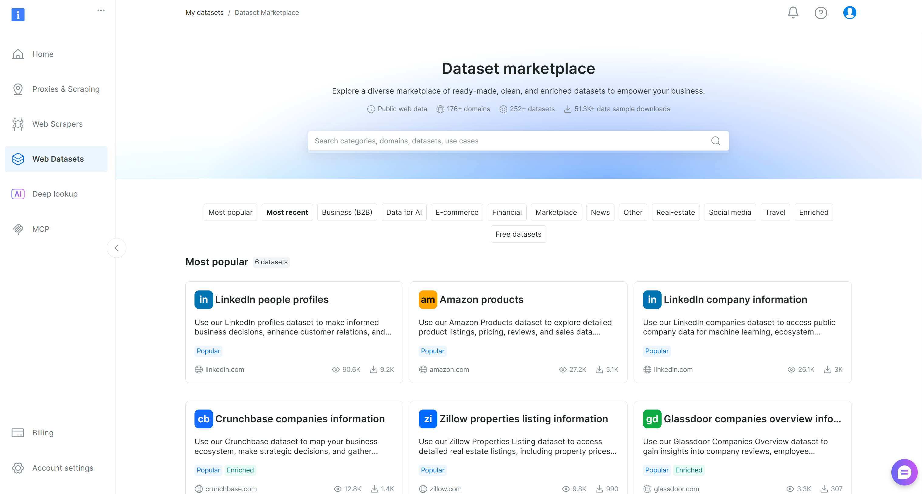
Here, you can explore 200+ scraped datasets from over 155 domains, containing billions of records.

Now, look for the “Glassdoor companies overview information” dataset and open its page:

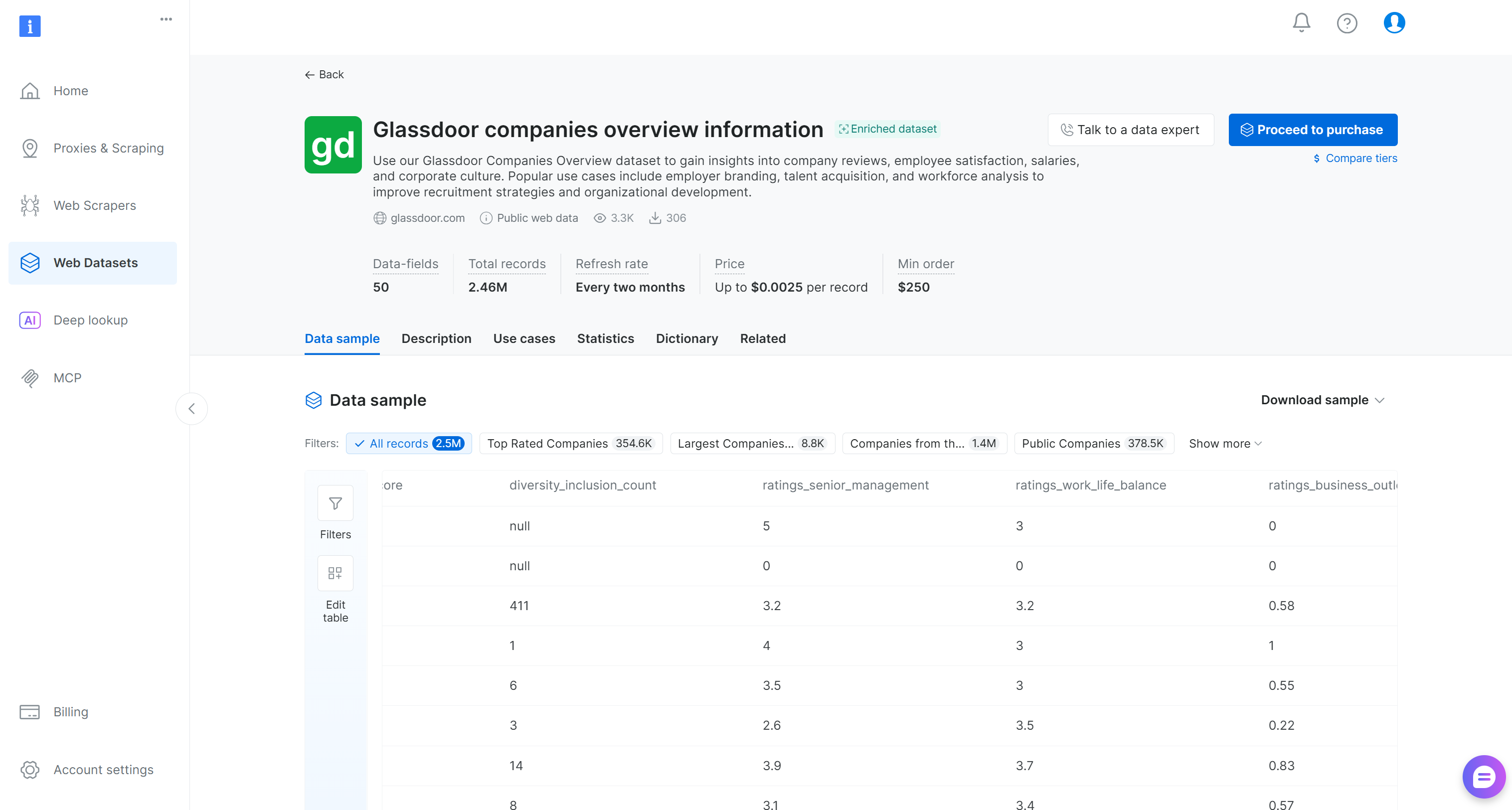
This dataset includes company reviews, employee satisfaction scores, salaries, and corporate culture information. Popular use cases include employer branding, talent acquisition, and workforce analysis. It contains over 2.46 million entries with 50 data fields.

You can choose to either purchase a filtered subset or download a free sample. In a production scenario, the larger the input dataset, the more reliable your feature engineering results will be.

For this tutorial, as it is just an example, we will count on the free sample. To get it, click the “Download sample” dropdown and select the “Download as JSON” option:

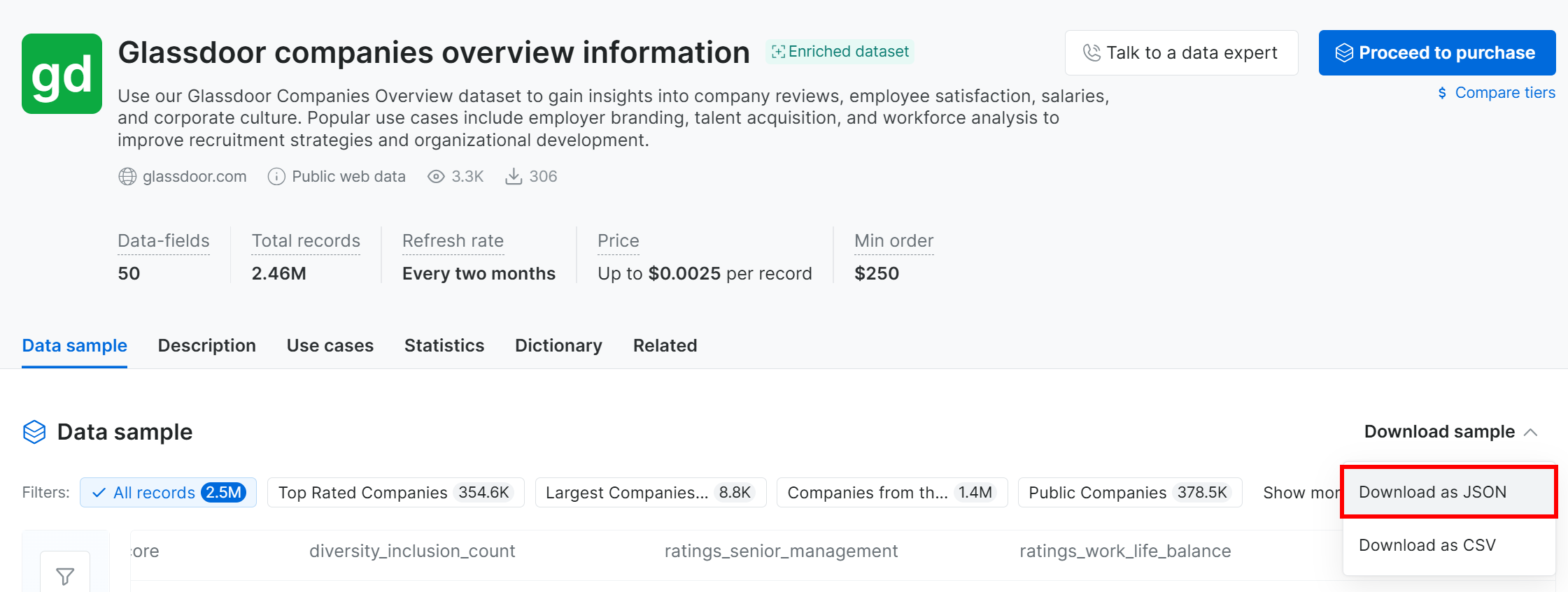
You will receive a sample file named Glassdoor companies overview information.json. This file contains 1,000 company records, each with 50 fields.

Rename the file to glassdoor-companies.json, and get ready to upload it to your S3 bucket. That will be used as input for your SageMaker feature engineering notebook. Well done!

Step #2: Upload the Web Data to Your S3 Bucket

Go to your Amazon S3 bucket page and click the “Upload” button to add the glassdoor-companies.json file. Once uploaded, it will appear in your bucket like this:

Alternatively, you can use one of the many Amazon S3 clients to upload the file.

Remember: With Bright Data Web Scraping APIs, you can send scraped data directly to Amazon S3.

Awesome! You now have some input web data for feature engineering in Amazon SageMaker.

Step #3: Get Started with Amazon SageMaker

Log in to the AWS Console and search for “SageMaker”. Select the service to open its main page:

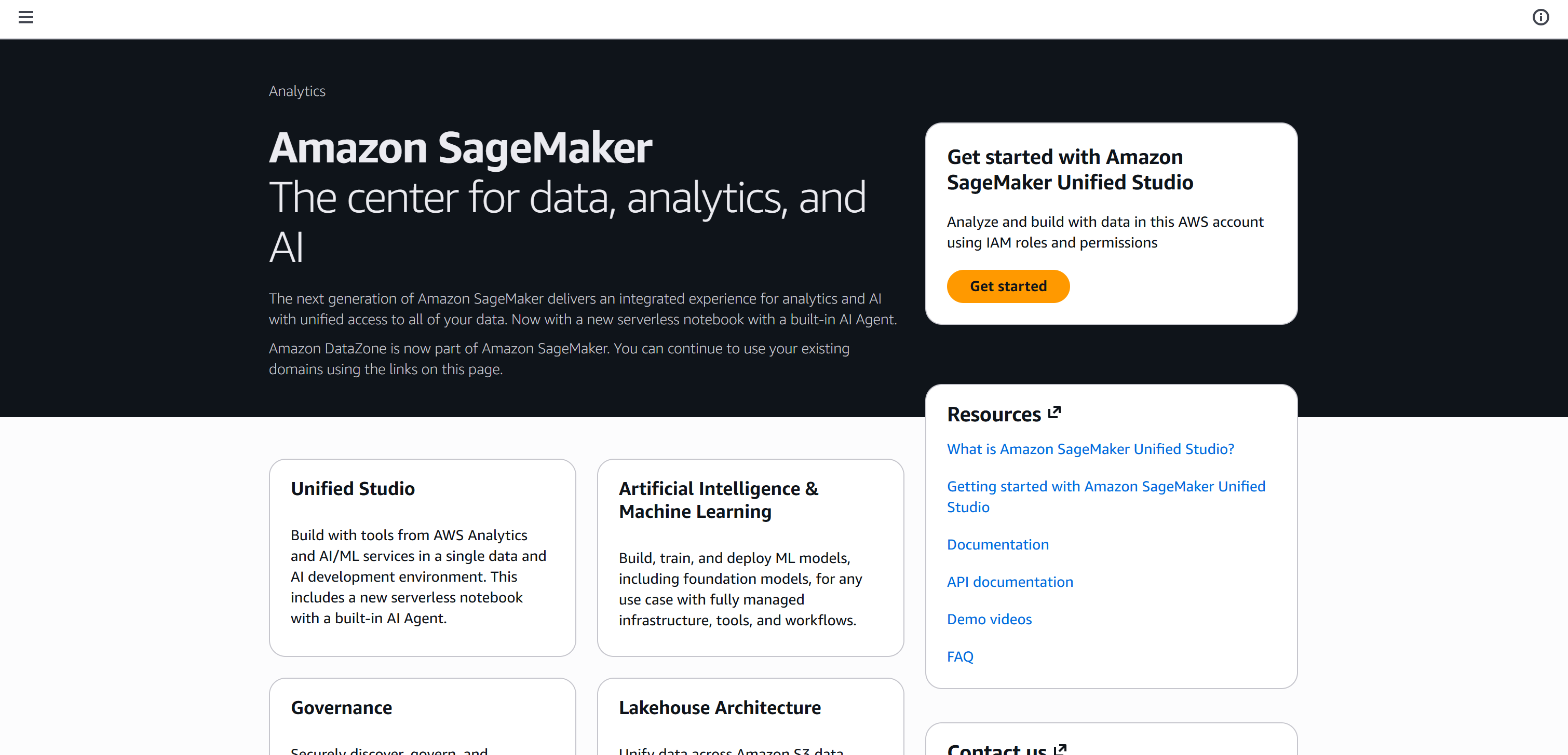
Click the “Get started” button to bootstrap your Amazon SageMaker experience.

On the setup page, for an automatic IAM setup, check that “Auto-create a new role with admin permissions” is selected. Continue by pressing the “Set up” button:

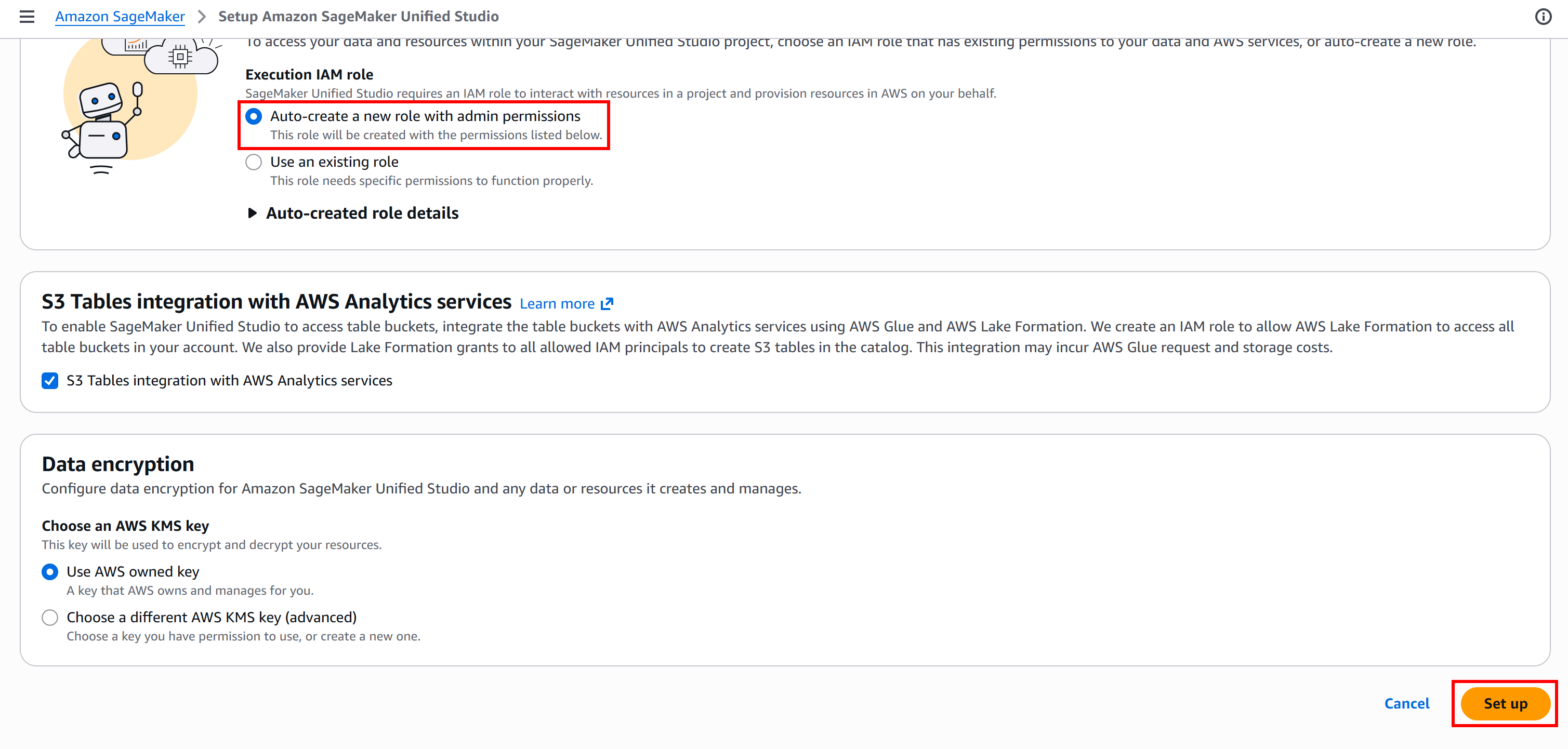
The initialization process may take a few minutes, so be patient. While it runs, you will see a “Setting up Amazon SageMaker Unified Studio…” message.

Once setup is complete, you will reach the following page:

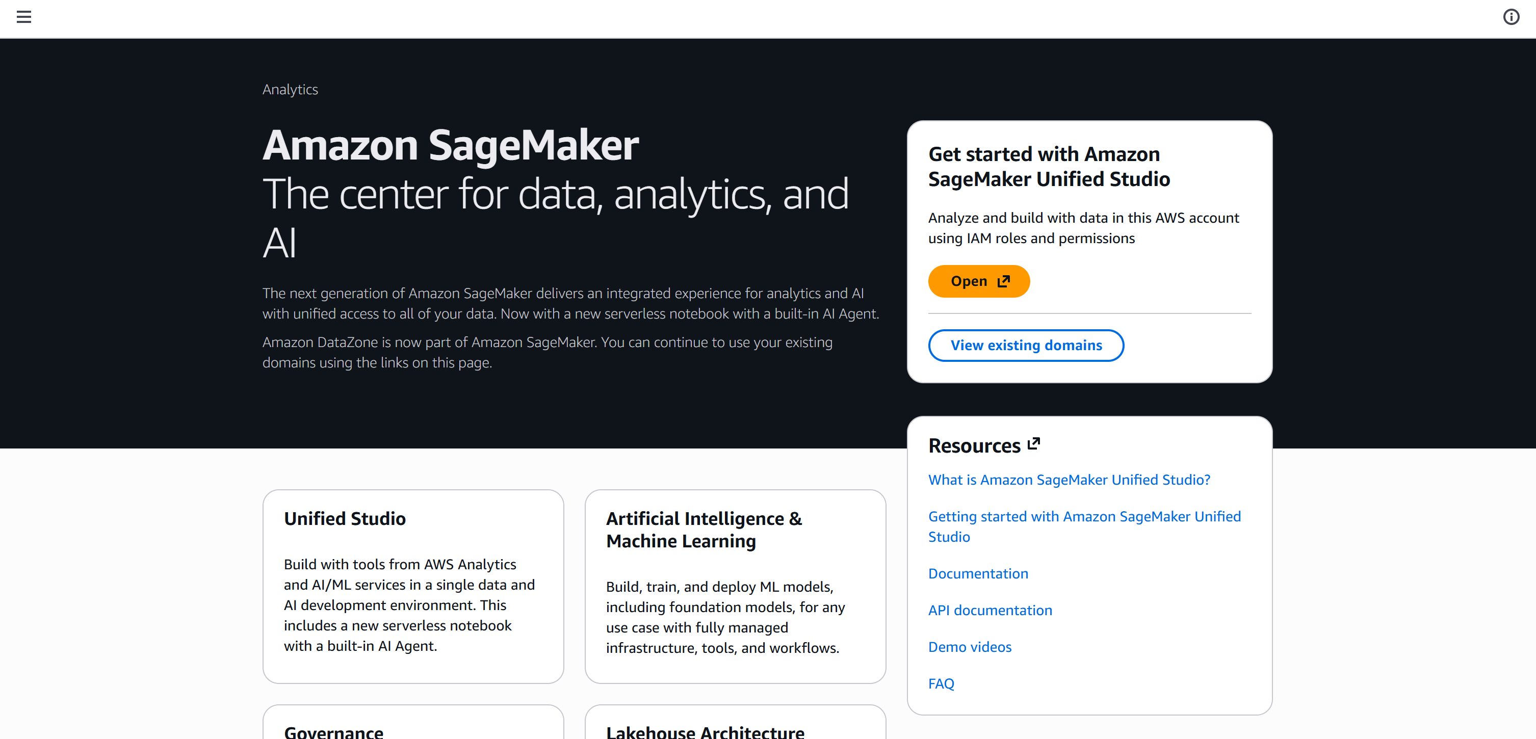
Click “Open” to launch Amazon SageMaker Unified Studio:

From here, you can explore and manage your SageMaker environment, including developing and running notebooks. Cool!

Step #4: Create a New Notebook

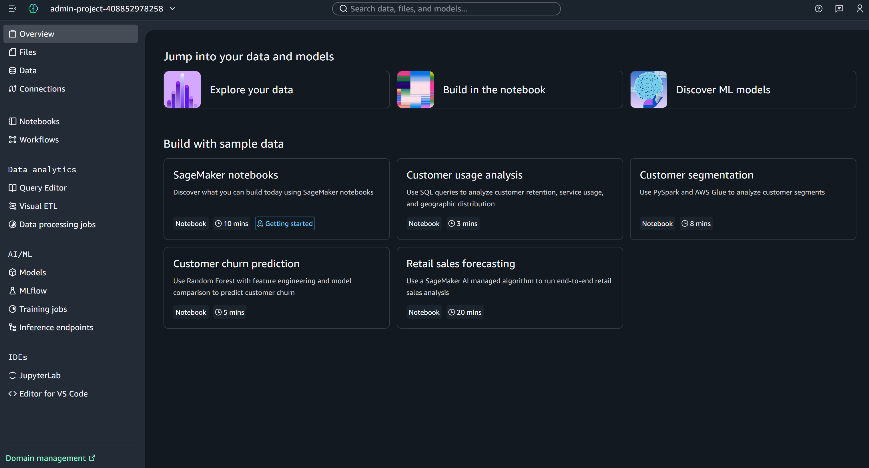
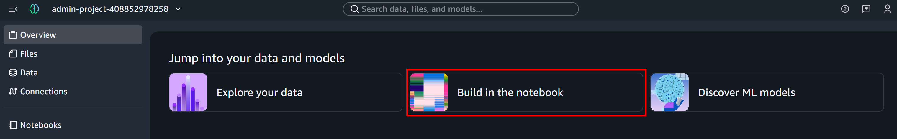
In Amazon SageMaker Unified Studio, click the “Build in the notebook” button to create a new notebook:

This is what your new SageMaker notebook should look like:

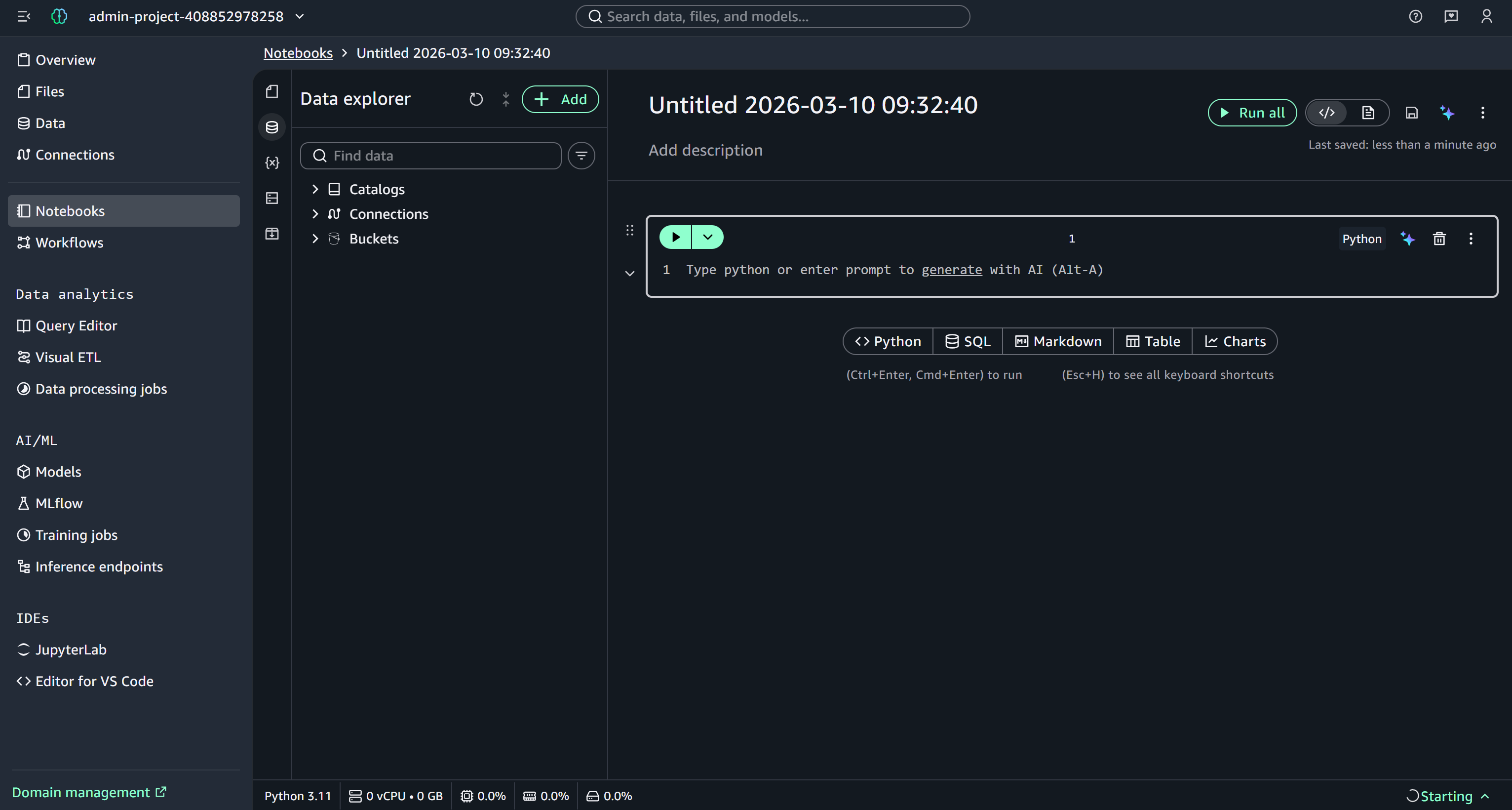
Consider giving your notebook a descriptive name, such as “Company Data Feature Engineering.”

An Amazon SageMaker notebook is a managed machine learning compute instance running Jupyter Notebook. It provides everything you need to prepare and process data, write and test training code, deploy models to SageMaker hosting, and validate your models.

Wonderful! You now have all the building blocks to implement the SageMaker feature engineering logic.

Step #5: Load the Input Web Data

The first step is to load your input Glassdoor web data from Bright Data into your SageMaker notebook.

In the “Data Explorer” panel on the left, expand the “Buckets” dropdown. Locate your S3 bucket and find the glassdoor-companies.json file. Click the burger menu next to the file and select the “Read as dataframe” option:

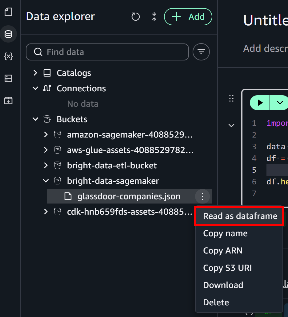
This will fill out the initial notebook cell with logic to load the file from S3:

import pandas as pd

data = pd.read_json("s3://bright-data-sagemaker/glassdoor-companies.json")

Note: Replace bright-data-sagemaker with the name of your S3 bucket.

Complete the data import logic in the first cell as follows:

import pandas as pd

# Load the input data from the S3 bucket
data = pd.read_json("s3://bright-data-sagemaker/glassdoor-companies.json")

# Normalize the structured JSON fields
df = pd.json_normalize(data.to_dict(orient="records"))

# Print the first 10 lines
df.head(10)

This code snippet loads and preprocesses a JSON dataset from an S3 bucket for analysis in Python. It uses pd.read_json() to read the file, then pd.json_normalize() to flatten nested JSON fields into a tabular DataFrame. Finally, df.head(10) displays the first 10 rows, giving a quick preview of the structured data.

Run the cell by pressing the “▶” button. You should see a preview like this:

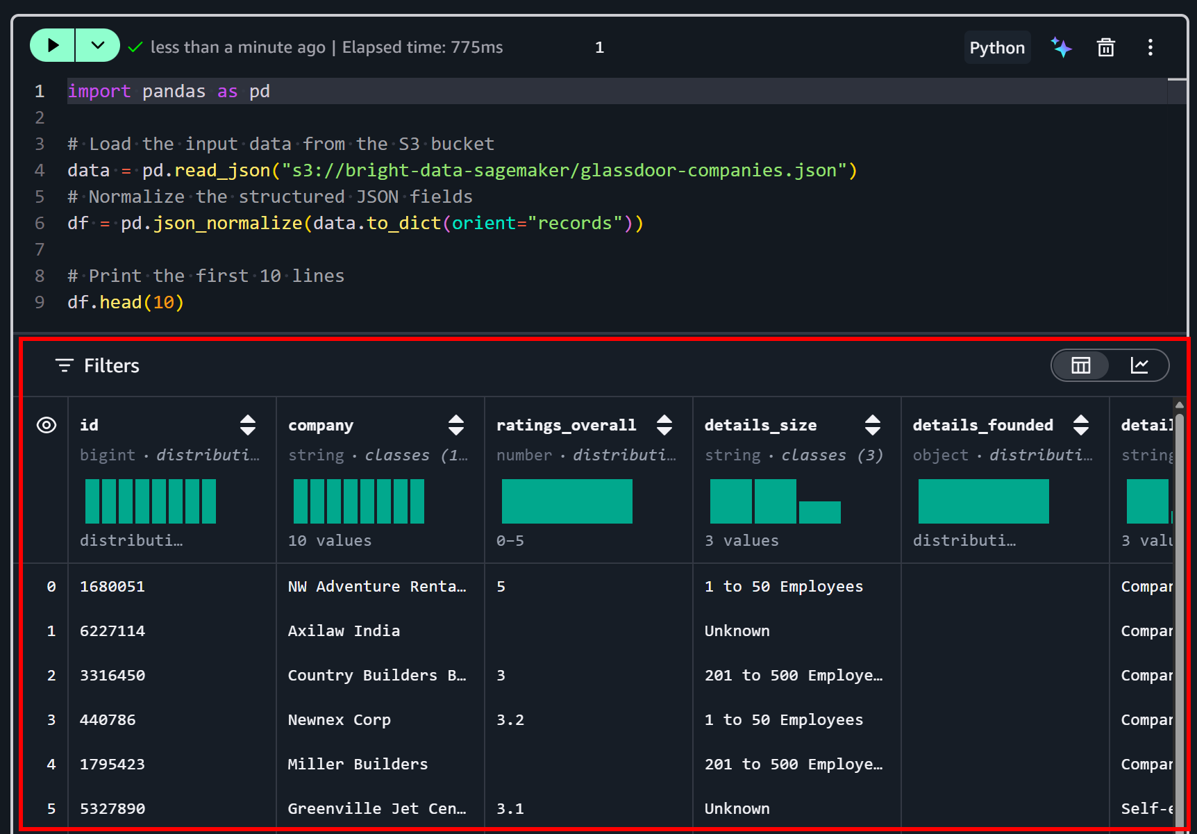
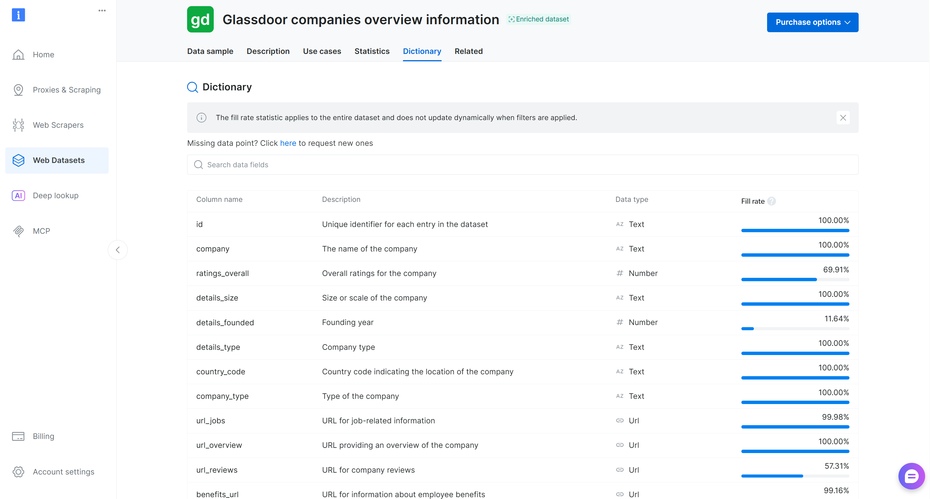
As you can tell, the dataset has been loaded correctly. This contains 50 data fields, as listed on the “Dictionary” tab on the Bright Data dataset page:

You have input web data ready for feature engineering. Fantastic!

Step #6: Pre-Process the Input Data

Now that you have imported your dataset into the notebook, the next step is to clean and prepare it for feature engineering.

Add a new cell in your SageMaker notebook and enter the following code:

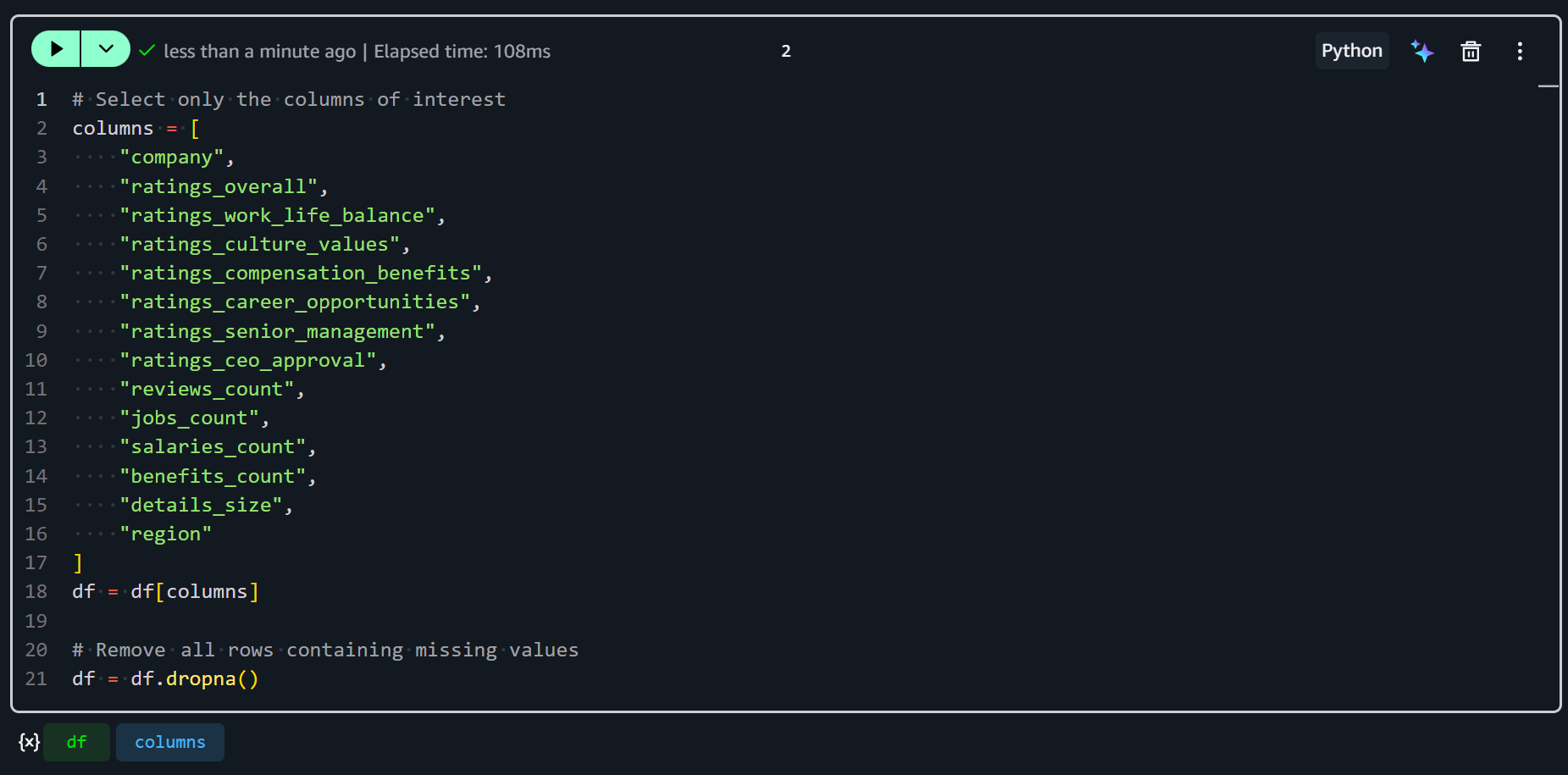
# Select only the columns of interest
columns = [
    "company",
    "ratings_overall",
    "ratings_work_life_balance",
    "ratings_culture_values",
    "ratings_compensation_benefits",
    "ratings_career_opportunities",
    "ratings_senior_management",
    "ratings_ceo_approval",
    "reviews_count",
    "jobs_count",
    "salaries_count",
    "benefits_count",
    "details_size",
    "region"
]
df = df[columns]

# Remove all rows containing missing values
df = df.dropna()

This snippet selects only the columns of interest, keeping your dataset focused on relevant metrics and identifiers. Then, it utilizes df.dropna() to remove any rows that contain missing values in the selected columns. This ensures that your data is clean and consistent for feature engineering.

Your new cell will look like this:

Great! Your input dataset is now ready for feature engineering in SageMaker.

Step #7: Define the Features

It is time to define the features you will use for machine learning. Remember that features are derived columns that summarize or transform raw data into meaningful metrics that better represent underlying patterns.

In this example, you will add features that capture company culture, compensation, popularity, and growth activity.

First, the culture_score feature combines multiple related ratings into a single metric that represents a company’s overall cultural environment:

df["culture_score"] = (
    df["ratings_culture_values"] +
    df["ratings_work_life_balance"] +
    df["ratings_senior_management"]
) / 3

It averages three rating columns:

• ratings_culture_values: Describes how well the company embodies its stated values.
• ratings_work_life_balance: Rates employees’ perception of work-life balance.
• ratings_senior_management: Tracks the perception of leadership and management.

Summing the three ratings and dividing by 3 produces a normalized score. The resulting score keeps the same scale as the original ratings and gives equal weight to each aspect of culture.

Second, the compensation_score feature represents a combined view of employee satisfaction with pay and career growth:

df["compensation_score"] = (
    df["ratings_compensation_benefits"] +
    df["ratings_career_opportunities"]
) / 2

It involves:

• ratings_compensation_benefits: Marks the employees’ satisfaction with pay and benefits.
• ratings_career_opportunities: Track the employees’ satisfaction with career advancement opportunities.

By averaging, the feature will be scaled consistently with other scores to balance both aspects equally.

Third, the review_popularity feature measures how frequently a company is reviewed on Glassdoor:

df["review_popularity"] = df["reviews_count"].apply(lambda x: x ** 0.5)

This is retrieved by applying a square root transformation to the number of reviews. Why the square root? Because review counts are often highly skewed (some companies have thousands of reviews, many have very few). Taking the square root reduces the impact of extremely high values and stabilizes variance, making it easier to process and analyze.

Fourth, the hiring_intensity feature estimates how actively a company is hiring relative to its review activity:

df["hiring_intensity"] = df["jobs_count"] / (df["reviews_count"] + 1)

It is calculated by dividing the number of open job listings (jobs_count) by the number of reviews plus 1 (to avoid division by zero for companies with no reviews).

Higher values indicate companies that are actively hiring compared to how many employees are leaving reviews. This can be a proxy for growth or expansion activity.

Put it all together, and you will get:

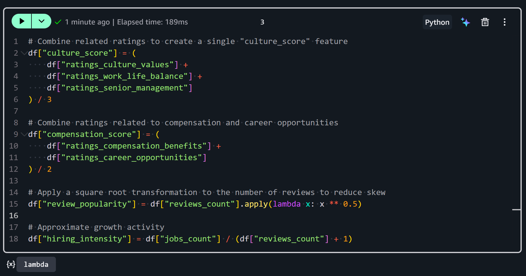
After running these transformations, your dataset now contains derived features that combine raw ratings and counts into more informative metrics. Sweet!

Step #8: Set the Target Variable

Now that your features are defined, the next step is to set the target variable for your machine learning task. The target variable represents the outcome you want your model to predict. In this case, you will predict whether a company has high employee satisfaction.

To set the target, add a new cell in your notebook and add this code:

# Define the target variable
df["high_satisfaction"] = (df["ratings_overall"] >= 4).astype(int)

This creates a Boolean field where companies with an overall rating of 4 or higher are marked as True (high satisfaction), and others as False (low satisfaction).

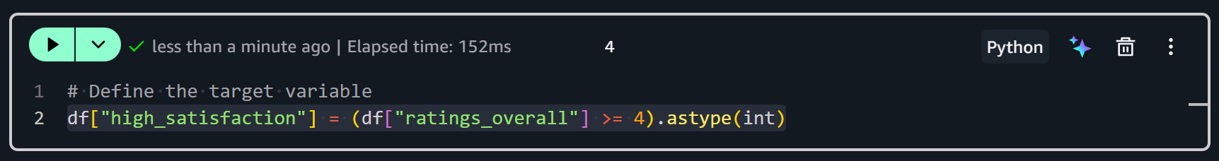
Many machine learning algorithms require a numeric target variable. By converting the satisfaction ratings into a binary 0/1 boolean label, you can train models for classification tasks. This helps you predict whether a company will likely have highly satisfied employees based on the features you created. Achieve that in the next step!

Step #9: Train the ML Model for Satisfaction Prediction

With your features and target variable defined, you can now train a machine learning model to predict high employee satisfaction.

The chosen ML model is XGBoost, a gradient boosting algorithm that performs exceptionally well on tabular data and classification tasks. It is good for predicting the high_satisfaction variable based on a mix of numerical and derived features.

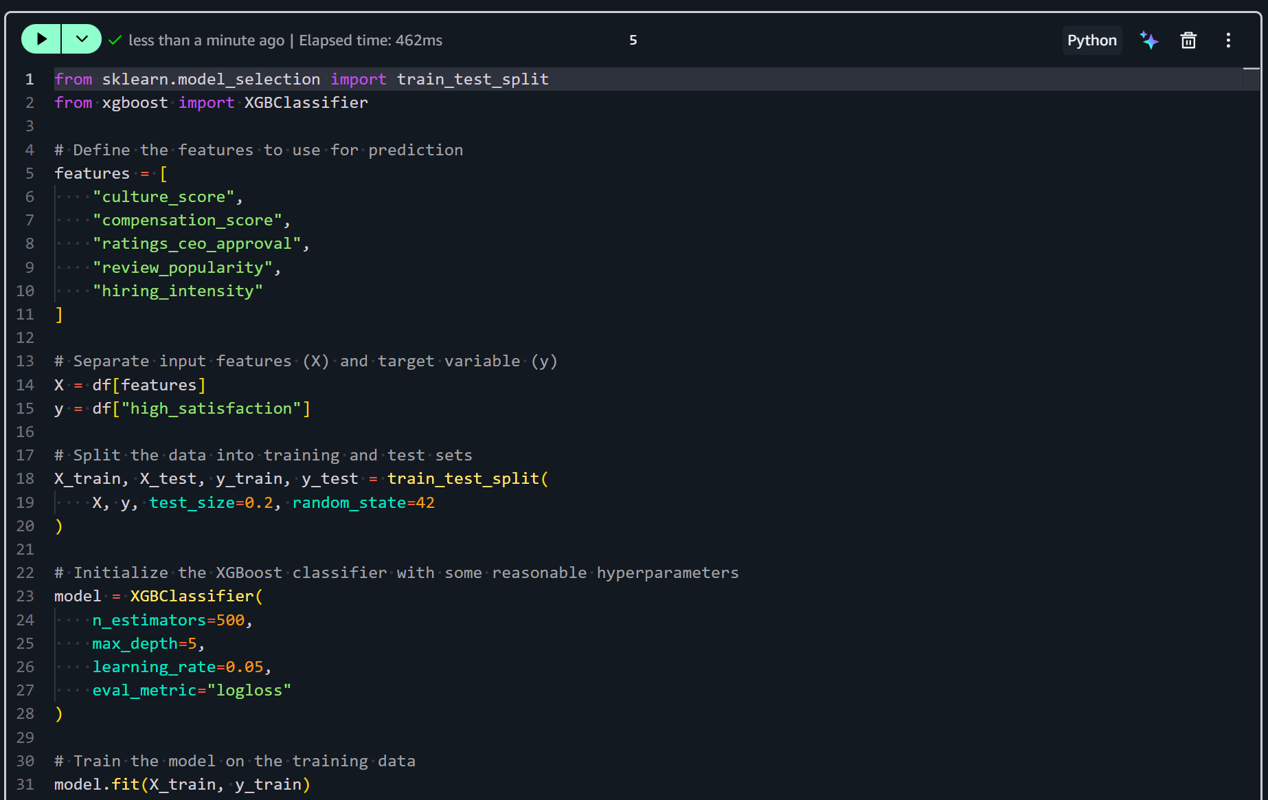
Add a new cell in your notebook and add the logic to train your model with:

from sklearn.model_selection import train_test_split
from xgboost import XGBClassifier

# Define the features to use for prediction
features = [
    "culture_score",
    "compensation_score",
    "ratings_ceo_approval",
    "review_popularity",
    "hiring_intensity"
]

# Separate input features (X) and target variable (y)
X = df[features]
y = df["high_satisfaction"]

# Split the data into training and test sets
X_train, X_test, y_train, y_test = train_test_split(
    X, y, test_size=0.2, random_state=42
)

# Initialize the XGBoost classifier with some reasonable hyperparameters
model = XGBClassifier(
    n_estimators=500,
    max_depth=5,
    learning_rate=0.05,
    eval_metric="logloss"
)

# Train the model on the training data
model.fit(X_train, y_train)

The above snippet prepares and trains a machine learning model to predict high employee satisfaction. It selects the engineered features and splits the data into training and test sets. Then, it initializes an XGBoost classifier with tuned hyperparameters. Finally, it fits the model to the training data.

Execute the cell to actually train the predictive model:

After this step, your XGBoost classifier is trained and ready for evaluation and prediction. The next step is to assess its performance!

Step #10: Evaluate the Model Performance

The final step is to assess how well your model performs on unseen data. Add a new cell in your notebook with this code:

from sklearn.metrics import classification_report
from sklearn.metrics import confusion_matrix, roc_auc_score, accuracy_score

# Use the trained model to predict labels on the test set
pred = model.predict(X_test)

print(classification_report(y_test, pred))

# Confusion matrix
cm = confusion_matrix(y_test, pred)
print("\nConfusion Matrix:\n", cm)

# ROC-AUC score
roc = roc_auc_score(y_test, model.predict_proba(X_test)[:,1])
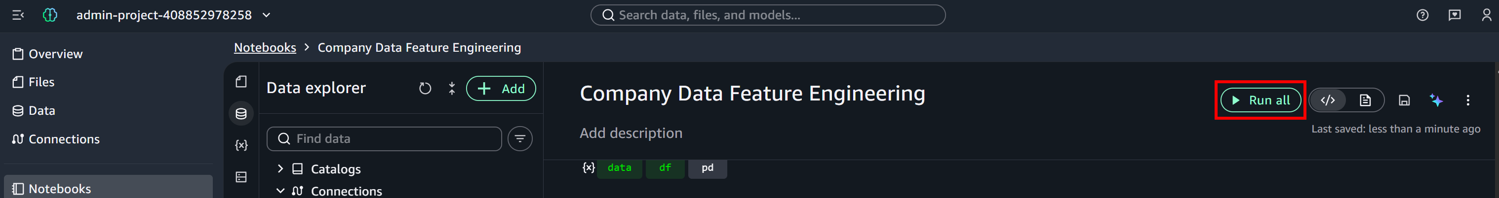
print("\nROC-AUC:", roc)

Press the “Run All” button to execute all steps and compute the metrics:

After the last cell executes, you should see output similar to this:

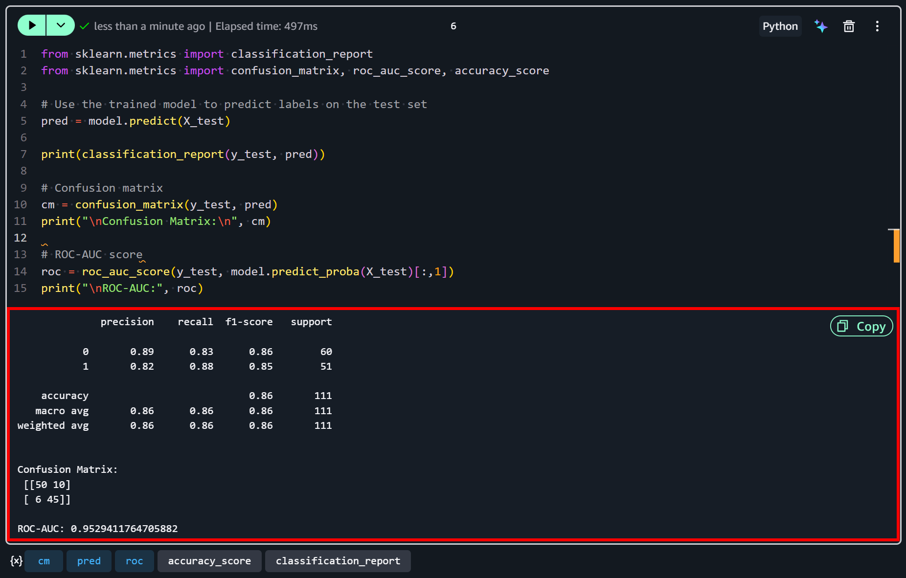
These results suggest that the model performs reasonably well for this example dataset. With an accuracy of 86% and a ROC-AUC of 0.95, it demonstrates a strong ability to discriminate between high- and low-satisfaction companies.

Both classes show balanced precision and recall, meaning the model is similarly effective at correctly identifying companies with high satisfaction (1) and those with lower satisfaction (0).

Yet, some misclassifications remain… As reflected in the confusion matrix, 10 low-satisfaction companies were incorrectly predicted as high-satisfaction, and 6 high-satisfaction companies were incorrectly predicted as low-satisfaction.

This indicates that while the model captures the main patterns in the data, it is not perfect and could be further improved with additional features (or more data).

Et voilà! Thanks to the Bright Data input web dataset, you were able to perform feature engineering and train a predictive model in Amazon SageMaker. This is just one of many use cases you could explore, thanks to the wide variety of structured web datasets offered by Bright Data.

Next Steps

The current model, which predicts high employee satisfaction using fields derived through feature engineering, achieves decent results. Still, there is room for improvement. There are several ways to enhance its performance, including:

• Create more derived features: Combine existing ratings in new ways. For example, you could calculate a leadership_score from ratings_senior_management and ratings_ceo_approval, or a work_life_compensation_ratio to capture trade-offs between pay and work-life balance. Explore ratios, differences, or interactions between features, which can reveal hidden patterns.
• Transform skewed distributions: Features like reviews_count or jobs_count are often skewed. We already applied a square root transform, but consider logarithmic or Box-Cox transformations to further stabilize variance.
• Incorporate categorical features: Currently, region and details_size are not numeric. Encoding them with one-hot encoding or target encoding could provide additional predictive signal.
• Aggregate multiple data points: If you can get historical review or hiring trends, creating features like average growth in jobs_count over time or change in culture_score could capture dynamic company behavior.
• Feature selection and importance analysis: After training, inspect XGBoost feature importance to identify which features contribute most to predictions. You may engineer new features inspired by the most predictive ones.
• External data enrichment: Consider merging other Bright Data datasets to create richer, contextual features.

Conclusion

In this tutorial, you saw what Amazon SageMaker brings to the table for machine learning scenarios. Specifically, you learned why scraped datasets are excellent sources for feature engineering and how they can be applied to train predictive ML models.

As demonstrated, Bright Data provides a rich dataset marketplace covering hundreds of domains and billions of web data records. These datasets are continuously updated through web scraping, making them ideal for supporting machine learning and AI workflows. Importantly, they integrate seamlessly with Amazon SageMaker, as illustrated in this guide.

Create a free Bright Data account today and start exploring our web data solutions!