How to Use Web Scraping for Machine Learning

In this guide, you will learn:

• What is machine learning?
• Why web scraping is useful for machine learning
• How to perform scraping for machine learning
• How to use machine learning on scraped data
• Details on the process of training ML models with scraped data
• How to set up ETLs when scraping data for machine learning

Let’s dive in!

What Is Machine Learning?

Machine learning, also known as ML, is a subsection of Artificial Intelligence (AI) that focuses on building systems capable of learning from data. In particular, the great revolution that comes from applying machine learning to software and computed systems is that computers do not need to be explicitly programmed to solve an ML problem. Thanks to machine learning systems learning from data.

How do machines can learn from data? Well, you can think of machine learning as nothing more than applied mathematics. The ML models, in fact, can identify the patterns of the underlying data they are exposed to, enabling them to make predictions on the outputs when exposed to new input data.

Why Web Scraping is Useful for Machine Learning

Machine learning systems—but, more in general, any AI system—need data to train the models, and this is where web scraping comes in as an opportunity for data professionals.

So here are some reasons why web scraping is important for machine learning:

• Data collection at scale: Machine learning models—and especially deep learning models—require vast amounts of data to train effectively. Web scraping allows for the collection of large-scale datasets that might not be available elsewhere.
• Diverse and rich data sources: If you already have data to train your ML models, scraping the web is an opportunity to enlarge your datasets, as the web hosts a wide multitude of data.
• Up-to-date information: Sometimes, the data you have is not updated with the latest trends, and here is where web scraping has you covered. In fact, for models that rely on the most recent information (e.g., stock price prediction, news sentiment analysis, etc.), web scraping can provide up-to-date data feeds.
• Enhancing model performance: The data you have may simply never enough—depending on the models or the project you are working on. For this reason, retrieving data from the web by using web scraping is a way to get more data with the purpose of enhancing your model’s performance and validating it.
• Market analysis: Scraping reviews, comments, and ratings helps in understanding consumer sentiment, which is valuable for businesses. It can also help in collecting data on emerging topics and can aid in forecasting market trends or public opinion.

Prerequisites

In this tutorial, you will learn how to perform web scraping for maching learning in Python.

To reproduce the Python project below, your system has to match the following prerequisites:

• Python 3.6 or higher: Any Python version higher than 3.6 will do. In particular, we will install the dependencies via pip which is already installed with any Python version greater than 3.4.
• Jupyter Notebook 6.x: We will use a Jupiter Notebook to analyze the data and make predictions with machine learning. Any version higher than 6.x will do.
• An IDE: VS CODE or any other Python IDE of your choice will do.

How to Perform Scraping for Machine Learning

In this step-by-step section, you will learn how to create a web scraping project that retrieves data to be further analyzed with machine learning.

In detail, you will see how to scrape Yahoo Finance to get NVIDIA stock prices. We will then use that data for maching learning.

Step #1: Setting up the environment

First of all, create a repository—called, for example, scraping_project—that has subfolders called data, notebooks, and scripts like so:

scraping_project/
├── data/
│   └── ...
├── notebooks/
│   └── analysis.ipynb
├── scripts/
│   └── data_retrieval.py
└── venv/

Where:

• data_retrieval.py will contain your scraping logic.
• analysis.ipynb will contain the maching learning logic.
• data/ will contain the scraped data to analyze via maching learning.

The venv/ folder contains the virtual environment. You can create it like so:

python3 -m venv venv 

To activate it, on Windows, run:

venv\Scripts\activate

On macOS/Linux, execute:

source venv/bin/activate

You can now install all the needed libraries:

pip install selenium requests pandas matplotlib scikit-learn tensorflow notebook

Step #2: Define the target page

To get the NVIDIA historical data, you have to go to the following URL:

https://finance.yahoo.com/quote/NVDA/history/

However, the page presents some filters that allow you to define how you want the data to be displayed:

To retrieve enough data for machine learning, you can filter them by 5 years. For your convenience, you can use the following URL that already filters the data by 5 years:

https://finance.yahoo.com/quote/NVDA/history/?frequency=1d&period1=1574082848&period2=1731931014

In this page, you have to target the following table and retrieve the data from it:

The CSS selector that defines the table is .table so you can write the following code in the data_retrieval.py file:

from selenium import webdriver
from selenium.webdriver.chrome.service import Service
from selenium.webdriver.support.ui import WebDriverWait
from selenium.webdriver.support import expected_conditions as EC
from selenium.webdriver.common.by import By
from selenium.common import NoSuchElementException
import pandas as pd
import os

# Configure Selenium
driver = webdriver.Chrome(service=Service())

# Target URL
url = "https://finance.yahoo.com/quote/NVDA/history/?frequency=1d&period1=1574082848&period2=1731931014"
driver.get(url)

# Wait for the table to load
try:
    WebDriverWait(driver, 20).until(
        EC.presence_of_element_located((By.CSS_SELECTOR, ".table"))
    )
except NoSuchElementException:
    print("The table was not found, verify the HTML structure.")
    driver.quit()
    exit()

# Locate the table and extract its rows
table = driver.find_element(By.CSS_SELECTOR, ".table")
rows = table.find_elements(By.TAG_NAME, "tr")

So far, this code does the following:

• Sets up a Selenium Chrome driver instance
• Defines the target URL and instruct Selenium to visit it
• Waits for the table to be loaded: In this case, the target table is loaded by Javascript, so the web driver waits 20 seconds, just to be sure the table is loaded
• Intercepts the whole table by using the dedicated CSS selector

Step #3: Retrieve the data and save them into a CSV file

At this point, you can do the following:

1. Extract the headers from the table (his will be appended as is into the CSV file)
2. Retrieve all the data from the table
3. Convert the data into a Numpy data frame

You can do this with the following code:

# Extract headers from the first row of the table
headers = [header.text for header in rows[0].find_elements(By.TAG_NAME, "th")]

# Extract data from the subsequent rows
data = []
for row in rows[1:]:
    cols = [col.text for col in row.find_elements(By.TAG_NAME, "td")]
    if cols:
        data.append(cols)

# Convert data into a pandas DataFrame
df = pd.DataFrame(data, columns=headers)

Step #4: Save the CSV file into the data/ folder

If you look at the folder structure created, you should remember that the data_retrieval.py file is in the scripts/ folder. The CVS file, instead, has to be saved into the data/ folder, so you have to consider this in your code:

# Determine the path to save the CSV file
current_dir = os.path.dirname(os.path.abspath(__file__))  

# Navigate to the "data/" directory
data_dir = os.path.join(current_dir, "../data") 

# Ensure the directory exists 
os.makedirs(data_dir, exist_ok=True)  

# Full path to the CSV file
csv_path = os.path.join(data_dir, "nvda_stock_data.csv")  

# Save the DataFrame to the CSV file
df.to_csv(csv_path, index=False)
print(f"Historical stock data saved to {csv_path}")

# Close the WebDriver
driver.quit()

This code determines the (absolute) current path using the method os.path.dirname(), navigates to the data/ folder with the method os.path.join(), ensures it exists with the method os.makedirs(data_dir, exist_ok=True), saves the data to a CSV file with the method df.to_csv() from the Pandas library, and finally quits the driver.

Step #5: Putting it all together

Here is the complete code for the data_retrieval.py file:

from selenium import webdriver
from selenium.webdriver.chrome.service import Service
from selenium.webdriver.support.ui import WebDriverWait
from selenium.webdriver.support import expected_conditions as EC
from selenium.webdriver.common.by import By
from selenium.common import NoSuchElementException
import pandas as pd
import os

# Configure Selenium
driver = webdriver.Chrome(service=Service())

# Target URL
url = "https://finance.yahoo.com/quote/NVDA/history/?frequency=1d&period1=1574082848&period2=1731931014"
driver.get(url)

# Wait for the table to load
try:
    WebDriverWait(driver, 5).until(
        EC.presence_of_element_located((By.CSS_SELECTOR, "table.table.yf-j5d1ld.noDl"))
    )
except NoSuchElementException:
    print("The table was not found, verify the HTML structure.")
    driver.quit()
    exit()

# Locate the table and extract its rows
table = driver.find_element(By.CSS_SELECTOR, ".table")
rows = table.find_elements(By.TAG_NAME, "tr")

# Extract headers from the first row of the table
headers = [header.text for header in rows[0].find_elements(By.TAG_NAME, "th")]

# Extract data from the subsequent rows
data = []
for row in rows[1:]:
    cols = [col.text for col in row.find_elements(By.TAG_NAME, "td")]
    if cols:
        data.append(cols)

# Convert data into a pandas DataFrame
df = pd.DataFrame(data, columns=headers)

# Determine the path to save the CSV file
current_dir = os.path.dirname(os.path.abspath(__file__))  

# Navigate to the "data/" directory
data_dir = os.path.join(current_dir, "../data") 

# Ensure the directory exists 
os.makedirs(data_dir, exist_ok=True)

# Full path to the CSV file  
csv_path = os.path.join(data_dir, "nvda_stock_data.csv")

# Save the DataFrame to the CSV file
df.to_csv(csv_path, index=False)
print(f"Historical stock data saved to {csv_path}")

# Close the WebDriver
driver.quit()

So, with a few lines of code, you retrieved 5 years of historical data on the NVIDIA stocks and saved them into a CSV file.

On Windows, launch the above script with:

python data_retrieval.py

Or equivalently, On Linux/macOS:

python3 data_retrieval.py

Below is how the output scraped data appears:

Using Machine Learning on Scraped Data

Now that the data is saved into a CSV file, you can use machine learning to make predictions.

Let’s see how you can do so in the following steps.

Step #1: Create a new Jupyter Notebook file

To create a new Jupyter Notebook file, navigate to the notebooks/ folder from the main one:

cd notebooks 

Then, open a Jupyter Notebook like so:

jupyter notebook

When the browser is open, click on New > Python3 (ipykernel) to create a new Jupyter Notebook file:

Rename the file, for example, as analysis.ipynb.

Step #2: Open the CSV file and show the head

Now you can open the CSV file containing the data and show the head of the data frame:

import pandas as pd

# Path to the CSV file
csv_path = "../data/nvda_stock_data.csv"

# Open the CVS file
df = pd.read_csv(csv_path)

# Show head
df.head()

This code goes to the data/ folder with csv_path = "../data/nvda_stock_data.csv". Then, it opens the CSV with the method pd.read_csv() as a data frame and shows its head (the first 5 rows) with the method df.head().

Here is the expected result:

Step #3: Visualize the trend over time of the** Adj Close value

Now that the data frame is correctly loaded, you can visualize the trend of the Adj Close value, which represents the adjusted closing value:

import matplotlib.pyplot as plt

# Ensure the "Date" column is in datetime forma
df["Date"] = pd.to_datetime(df["Date"])

# Sort the data by date (if not already sorted)
df = df.sort_values(by="Date")

# Plot the "Adj Close" values over time
plt.figure(figsize=(10, 6))
plt.plot(df["Date"], df["Adj Close"], label="Adj Close", linewidth=2)

# Customize the plot
plt.title("NVDA Stock Adjusted Close Prices Over Time", fontsize=16) # Sets title
plt.xlabel("Date", fontsize=12) # Sets x-axis label
plt.ylabel("Adjusted Close Price (USD)", fontsize=12) # Sets y-axis label
plt.grid(True, linestyle="--", alpha=0.6) # Defines styles of the line
plt.legend(fontsize=12) # Shows legend
plt.tight_layout()

# Show the plot
plt.show()

This snippet does the following:

• df["Date"] accesses the Date column of the data frame and, with the method pd.to_datetime(), ensures that the dates are in the date format
• The df.sort_values() sorts the dates of the Date column. This ensures the data will be displayed in chronological order.
• plt.figure() sets the dimensions of the plot and plt.plot() displays it
• The lines of code under the # Customize the plot comment are useful to customize the plot by providing the title, the labels of the axes, and displaying the legend
• The plt.show() method is the one that actually allows the plot to be displayed

The expected result is something like that:

This plot shows the actual trend of the adjusted closed values over time of the NVIDIA stocks values. The machine learning model you will be training will have to predict them as best as it can.

Step #3: Preparing data for machine learning

Time to prepare the data for machine learning!

First, you can do data cleaning and preparation:

from sklearn.preprocessing import MinMaxScaler

# Convert data types
df["Volume"] = pd.to_numeric(df["Volume"].str.replace(",", ""), errors="coerce")
df["Open"] = pd.to_numeric(df["Open"].str.replace(",", ""), errors="coerce")

# Handle missing values 
df = df.infer_objects().interpolate() 

# Select the target variable ("Adj Close") and scale the data
scaler = MinMaxScaler(feature_range=(0, 1))  # Scale data between 0 and 1
data = scaler.fit_transform(df[["Adj Close"]])

This code does the following:

• Converts the Volume and Open values with the method to_numeric()
• Handles missing values by using interpolation to fill them with the method interpolate()
• Scales the data with the MinMaxScaler()
• Selects and transforms (scales it) the target variable Adj Close with the method fit_transform()

Step #4: Create the train and test sets

The model used for this tutorial is an LSTM (Long Short-Term Memory), which is a RNN (Recurrent Neural Network), so create a sequence of steps to allow it to learn the data:

import numpy as np

# Create sequences of 60 time steps for prediction
sequence_length = 60
X, y = [], []

for i in range(sequence_length, len(data)):
    X.append(data[i - sequence_length:i, 0])  # Last 60 days
    y.append(data[i, 0])  # Target value

X, y = np.array(X), np.array(y)

# Split into training and test sets
split_index = int(len(X) * 0.8)  # 80% training, 20% testing
X_train, X_test = X[:split_index], X[split_index:]
y_train, y_test = y[:split_index], y[split_index:]

This code:

• Creates a sequence of 60 time steps. X is the array of the features, y is the array of the target value
• Splits the initial data frame like so: 80% becomes the train set, 20% the test set

Step #5: Train the model

You can now train the RNN on the train set:

from tensorflow.keras.models import Sequential
from tensorflow.keras.layers import Dense, LSTM

# Reshape X for LSTM [samples, time steps, features]
X_train = X_train.reshape((X_train.shape[0], X_train.shape[1], 1))
X_test = X_test.reshape((X_test.shape[0], X_test.shape[1], 1))

# Build the Sequential Neural Network
model = Sequential()
model.add(LSTM(32, activation="relu", return_sequences=False))
model.add(Dense(1))
model.compile(loss="mean_squared_error", optimizer="adam")

# Train the Model
history = model.fit(X_train, y_train, epochs=20, batch_size=32, validation_data=(X_test, y_test), verbose=1)

This code does the following:

• Respahes the array of the features to be ready for the LSTM neural network by using the method reshape(), both for the train and test sets
• Builds the LSTM neural network by setting its parameters
• Fits the LSTM to the train set by using the method fit()

So, the model has now fitted the train set and it is ready to make predictions.

Step #6: Make predictions and evaluate the model performance

The model is now ready to predict the Adj Close values and you can evaluate its performance like so:

from sklearn.metrics import mean_squared_error, r2_score

# Make Predictions
y_pred = model.predict(X_test)

# Inverse scale predictions and actual values for comparison
y_test = scaler.inverse_transform(y_test.reshape(-1, 1))
y_pred = scaler.inverse_transform(y_pred)

# Evaluate the Model
mse = mean_squared_error(y_test, y_pred)
r2 = r2_score(y_test, y_pred)

# print results
print("\nLSTM Neural Network Results:")
print(f"Mean Squared Error: {mse:.2f}")
print(f"R-squared Score: {r2:.2f}")

This code does the following:

• Inverses the values on the horizontal axis so that the data can be lately presented in chronological order. This is done with the method inverse_transform().
• Evaluates the model by using the mean squared error and the R^2 score.

Considering the statistical errors that can occur due to the stochastical nature of ML models, the expected result is something like so:

These are pretty good values, indicating the model chosen is a good one to predict the Adj Closegiven its features.

Step #7: Compare actual vs predicted values with a plot

When it comes to machine learning, comparing the results analytically—as we did in the previous step—can sometimes be not enough. To improve the chances that the model chosen is a good one, a typical solution is to also create a plot.

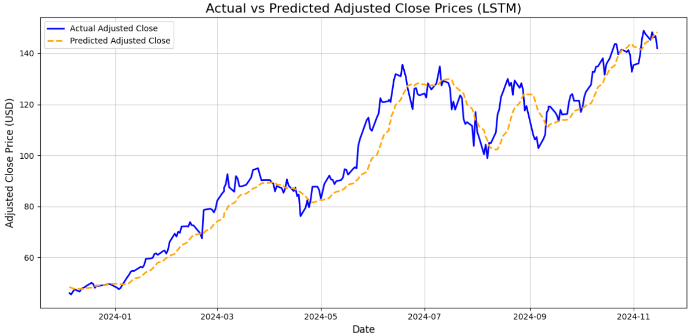
For example, a common solution is to create a plot that compares the actual values of the Adj Close with the predicted ones by the LSTM model:

# Visualize the Results
test_results = pd.DataFrame({
    "Date": df["Date"].iloc[len(df) - len(y_test):],  # Test set dates
    "Actual": y_test.flatten(),
    "Predicted": y_pred.flatten()
})

# Setting plot
plt.figure(figsize=(12, 6))
plt.plot(test_results["Date"], test_results["Actual"], label="Actual Adjusted Close", color="blue", linewidth=2)
plt.plot(test_results["Date"], test_results["Predicted"], label="Predicted Adjusted Close", color="orange", linestyle="--", linewidth=2)
plt.title("Actual vs Predicted Adjusted Close Prices (LSTM)", fontsize=16)
plt.xlabel("Date", fontsize=12)
plt.ylabel("Adjusted Close Price (USD)", fontsize=12)
plt.legend()
plt.grid(alpha=0.6)
plt.tight_layout()
plt.show()

This code:

• Sets the comparison of the actual and predicted values on the level of the test set, so the actual values have to be trimmed to the shape that the test set has. This is done with the methods iloc() and flatten().
• Creates the plot, adds labels to the axes, and the title, and manages other settings to improve the visualization.

The expected result is something like this:

As the plot shows, the values predicted by the LSTM neural network (yellow dotted line) predict pretty well the actual values (continuous blue line). This was respectable as the analytical results were good, but the plot surely helps visualize that the result is good indeed.

Step #8: Putting it all together

Here is the complete code for the analysis.ipynb notebook:

import numpy as np
import pandas as pd
import matplotlib.pyplot as plt
from sklearn.preprocessing import MinMaxScaler
from sklearn.metrics import mean_squared_error, r2_score
from tensorflow.keras.models import Sequential
from tensorflow.keras.layers import Dense, LSTM

# Path to the CSV file
csv_path = "../data/nvda_stock_data.csv"  
# Open CSV as data frame
df = pd.read_csv(csv_path)

# Convert "Date" to datetime format
df["Date"] = pd.to_datetime(df["Date"])

# Sort by date
df = df.sort_values(by="Date")

# Convert data types
df["Volume"] = pd.to_numeric(df["Volume"].str.replace(",", ""), errors="coerce")
df["Open"] = pd.to_numeric(df["Open"].str.replace(",", ""), errors="coerce")

# Handle missing values 
df = df.infer_objects().interpolate()

# Select the target variable ("Adj Close") and scale the data
scaler = MinMaxScaler(feature_range=(0, 1))  # Scale data between 0 and 1
data = scaler.fit_transform(df[["Adj Close"]])

# Prepare the Data for LSTM
# Create sequences of 60 time steps for prediction
sequence_length = 60
X, y = [], []

for i in range(sequence_length, len(data)):
    X.append(data[i - sequence_length:i, 0])  # Last 60 days
    y.append(data[i, 0])  # Target value

X, y = np.array(X), np.array(y)

# Split into training and test sets
split_index = int(len(X) * 0.8)  # 80% training, 20% testing
X_train, X_test = X[:split_index], X[split_index:]
y_train, y_test = y[:split_index], y[split_index:]

# Reshape X for LSTM [samples, time steps, features]
X_train = X_train.reshape((X_train.shape[0], X_train.shape[1], 1))
X_test = X_test.reshape((X_test.shape[0], X_test.shape[1], 1))

# Build the Sequential Neural Network
model = Sequential()
model.add(LSTM(32, activation="relu", return_sequences=False))
model.add(Dense(1))
model.compile(loss="mean_squared_error", optimizer="adam")

# Train the Model
history = model.fit(X_train, y_train, epochs=20, batch_size=32, validation_data=(X_test, y_test), verbose=1)

# Make Predictions
y_pred = model.predict(X_test)

# Inverse scale predictions and actual values for comparison
y_test = scaler.inverse_transform(y_test.reshape(-1, 1))
y_pred = scaler.inverse_transform(y_pred)

# Evaluate the Model
mse = mean_squared_error(y_test, y_pred)
r2 = r2_score(y_test, y_pred)

# Print results
print("\nLSTM Neural Network Results:")
print(f"Mean Squared Error: {mse:.2f}")
print(f"R-squared Score: {r2:.2f}")

# Visualize the Results
test_results = pd.DataFrame({
    "Date": df["Date"].iloc[len(df) - len(y_test):],  # Test set dates
    "Actual": y_test.flatten(),
    "Predicted": y_pred.flatten()
})

# Setting plot
plt.figure(figsize=(12, 6))
plt.plot(test_results["Date"], test_results["Actual"], label="Actual Adjusted Close", color="blue", linewidth=2)
plt.plot(test_results["Date"], test_results["Predicted"], label="Predicted Adjusted Close", color="orange", linestyle="--", linewidth=2)
plt.title("Actual vs Predicted Adjusted Close Prices (LSTM)", fontsize=16)
plt.xlabel("Date", fontsize=12)
plt.ylabel("Adjusted Close Price (USD)", fontsize=12)
plt.legend()
plt.grid(alpha=0.6)
plt.tight_layout()
plt.show()

Note that this whole code goes directly to the goal, skipping the parts showing the head of the data frame when opening it and plotting only the Adj Close actual values.

These steps were reported at the beginning of this paragraph as part of the preliminary data analysis, and are useful to understand what you are doing with the data before actually going to train an ML model.

NOTE: The code has been presented piece-by-piece but, considering the stochastic nature of ML, the suggestion is to run the whole code altogether to properly train and validate the LSTM model. Otherwise, the resulting final plot may be significantly different.

Notes on The Process of Training ML Models with Scraped Data

For the sake of simplicity, the step-by-step guide provided in this article goes directly on fitting an LSTM neural network.

In reality, this is not what happens with ML models. So, when you try to solve a problem that needs an ML model, the process is the following:

• Preliminary data analysis: This is the most important part of the process because is where you understand the data you have, do data cleaning by removing NaN values, manage eventual duplicates, and solve other mathematical problems related to the data you have.
• Training ML models: You never know if the first model you have in mind will be the best one to solve the problem you are facing with ML. A typical solution is to perform the so-called spot-check which means:
  • Training 3-4 ML models on the train set, and evaluate how they perform on that.
  • Getting the 2-3 ML models that best perform on the train set, and tune their hyperparameters.
  • Comparing the performance of the best models with tuned hyperparameters on the test set.
  • Choosing the one that performs best on the test set.
• Deployment: The model that performs best is, then, the one that will be deployed into production.

Setting Up ETLs When Scraping Data for Machine Learning

At the beginning of this article, we defined why web scraping is useful for machine learning. However, you may have noticed an incoherence in the project developed that relies on the fact that the data retrieved via web scraping have been saved into a CSV file.

This is a common practice in machine learning, but you should consider that it is better to do so at the beginning of an ML project, when the purpose is to find the best model that can predict future values of the target values.

When the best model is found, the subsequent practice is to set up an ETL (Extract Transform Load) pipeline to retrieve new data from the web, clean it, and load it into a database.

The process can be something like this:

• Extract: This phase retrieves the data from various sources, including the web via scaping
• Transform: The data collected undergo the process of data cleaning and preparation
• Load: The data retrieved and transformed are processed and saved into a database or a data warehouse

After the data are stored, the subsequent phase provides the integration with the machine learning workflows that, among other things, re-train the model on new data, and re-validate it.

Conclusion

In this article, we have shown how to retrieve data from the web via scraping and how to use them for machine learning purposes. We have, also, presented the importance of web scraping for machine learning and we have discussed the process of training and structuring ETLs.

While the project proposed is a simple one, it is understandable that the underlying processes— especially, those related to structuring ETLs to retrieve data from the web continuously to improve the ML model—introduce complexities that should be further analyzed.

Scraping Yahoo Finance in real-world scenarios can be far more complex than what has been shown here. The site employs some anti-scraping technologies, requiring extra attention. For a professional, full-featured, all-in-one solution, check out Bright Data’s Yahoo Finance Scraper!

If scraping is not your forte but you still need data for machine learning projects, explore our solutions for efficient data retrieval tailored to AI and machine learning needs.

Create a free Bright Data account today to try our scraper APIs or explore our datasets.